
Users frequently find their explorer spaces and exploration views displaying outdated information. Indeed this can happen if the source data is not ready when the indexing process is scheduled to start at a fixed time, so a manual re-run is needed when the data is available to ensure data freshness. Unfortunately scheduling explorer spaces is not possible in the current 3.x or 4.x versions of SAP BusinessObjects BI, but a workaround has been recently applied in one of our customers which we detail in this article.
Managing ETL dependencies with SAP BusinessObjects Data Services (Part 4)
Are you satisfied with the way you currently manage the dependencies in your ETL? In the part 1 of this article, I talked about the features I’m expecting from a dependency management system, and what are the main possibilities offered (directly or indirectly) by Data Services. In part 2, I proposed an architecture (structure and expected behavior) for a dependency management system inside Data Services. In part 3, I explained the complete implementation details. In this final part, I'm going to give you a feedback on how it went “in real life” as well as possible improvements. So, the most important question is of course "Does it work?". I'm happy to confirm that yes, it does! And it makes quite a difference in the life of the customer's Data Services administrator. Of course it doesn't change anything if the ETL is running fine, but when there are problems, this dependency management system can be a huge time-saver!
Informatica PowerCenter - Automated loop execution with exchange of input parameters
One often required functionality that's not inherent to any Informatica PowerCenter entity is to automate loop execution of arbitrary logic with exchange of input parameters. In this article I will give you the implementation steps so you can achieve this. Most common implementation occurs with execution of arbitrary Data Integration process for a time period that's comprised of multiple temporal scopes of a single process run. For example, reloading a full month of transactions after the cutoff date when retroactive bookings for previous month become impossible, by means of daily transaction increment.
Not missing a hit in SAP BusinessObjects using HTTP traffic logs
Monitoring the number of views of an important corporate document is a key need for any company who is aiming for better resource management and company-wide alignment. This is especially important in a migration project in order to define what content to migrate or in a document maintenance process to prioritize assignments. SAP BusinessObjects Auditing is able to register when documents are viewed or retrieved but it has certain limitations, so most of the users activity is lost. This article explains an alternative method to collect the number of views of any SAP BusinessObjects file type or web page that sits on our web server so they can complement our current auditing reports.
Managing ETL dependencies with SAP BusinessObjects Data Services (Part 3)
Are you satisfied with the way you currently manage the dependencies in your ETL? In Part 1 of this series, I talked about the features I expect from a dependency management system, and what are the main possibilities offered (directly or indirectly) by Data Services. In Part 2, I proposed an architecture (structure and expected behavior) for a dependency management system inside Data Services. Now I will give you the implementation details, while a feedback on how it went “in real life” as well as possible improvements will come in part 4. So how do we implement this theoretical solution in Data Services?
Common SAP Dashboards (Xcelsius) bugs and how to solve them
This post is about SAP BusinessObjects Dashboards (formerly known as Xcelsius) and its intricate form of work. If you are an assiduous dashboard developer or just beginning to work with the tool, you will notice some bugs that interfere with your developing and slows you down. My main goal is to talk about the bugs or "misfortunes" that I have commonly faced in SAP BO Dashboards (Xcelsius) and the workarounds that I have found to save you some time when working with this tool. My second objective is to open a discussion where you can comment on other SAP Dashboards issues and solutions you found.
Dashboard integration in SAP Crystal Reports
In this blog article I would like to share with you how to embed a dashboard in a Crystal Report using flash variables. First of all let’s give a scenario that leads us to do that. In this case we wanted to create a dashboard for a SAP GRC module. The problem was that we could not connect to the system directly with SAP BusinessObjects Dashboards (Xcelsius for the most nostalgic ones). Apart from that, there is a good thing about having a dashboard embedded in Crystal, you will have a dashboard that can be refreshed from Crystal Reports without needing a previous authentication. You will also be able to save the “report” (you can show the dashboard) in PDF with saved data and the dashboard will be completely clickable and navigable.
How to load and read Web Services Data Store in Data Integrator
On this article I will teach you in 12 steps how to load and read the information retrieved by a WebService based on a Java Application as a source of information. This is has a very important feature if for example you are building Java Social Media applications that read information from the Internet or if you have constructed a Java application that retrieves information in Json Structure XML. I will show you how Data Services makes requests and interprets replies from a web service Data Source.
If you need background information on the first steps of my process, I have done a first post on how to use Data Services SDK libraries to construct an AWTableMetadata in a Java application, followed by the post where I explained how to access a JAVA application as a source of information using the WebService DataStore in SAP Data Services.
If you already read my previous blogs, lets jump into how to load and read Web Services Data Store in Data Integrator.
Step 1:
Open Data Services Designer. Go to the Data Store perspective and right click with the mouse and select New.
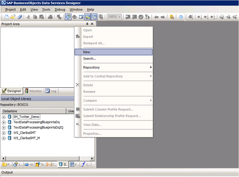
Picture1
Step 2:
Set the name of the extractor and the URL where your web service WSDL is located (see my previous blog for reference).
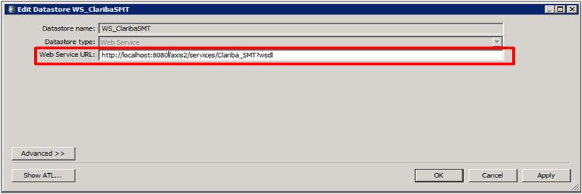
Picture2
Step 3:
Right Click on the “f(x)” symbol and select Import. Choose the functions from the webservice that you are going to use. In this example we select “getTableTweeetsEN” and “getTableTweeetsES”.

Picture3
Special Note:
To access to these functions inside a transformation we have to use the function call Schema provided by Data Services. In this case the function getTableTweets_EN receive an input and returns a table (AWTableMetadata table). This return type comes in an especial nested form from our Web Service. We will have to resolve this nested schema doing a couple of transformations below.
Picture4
Step 4:
Select the input parameter for the functions; in this case it is a field from a table called “WS_Parameter”. We select that table as a Source table and our first item in our data flow.
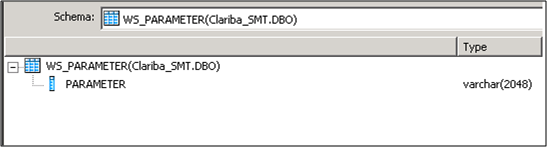
Picture5
Step 5:
Insert a transformation in the data flow as your second item. In this first query (Query1_EN). We create a SCHEMA called Schema 1, and assign the field came from the database “Parameter” as an attribute of this Schema.

Picture6
Step 6:
Create a second transformation (Query2_EN). This query will be in charge of calling the web service with the input parameter using the Function Call procedure. Right click on the Schema Table called Query2 and select new Function Call.
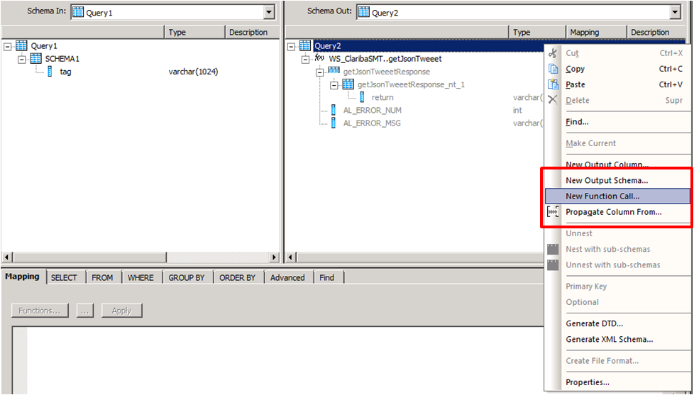
Picture7
Step 7:
Select the WS_ClaribaSMT dataSotre in the left panel, the right panel shows the functions that we imported to the Data Store. We select the first one getJsonTweet (For English Language) and click next.
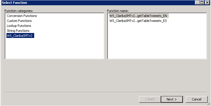
Picture8
Step 8:
We have to map the new function call Schema with the new Schema1. This is the structure used to call a Web Service in Data Services. In this case we are calling the function getJsonTweets_EN with a parameter nombre. Structure that matches our SHEMA1. Then click Finish.

Picture9
The final result will contain the function call. You can add also an attribute below the function call. In this case we add “load_date” containing the sysdate representing the date of the load data.

Picture10
Step 9:
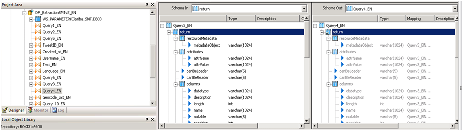
The third query will be in charge of the recognition of the data returned by the Web service. In this case the Schema is in the left panel. To capture this on Data integrator we need to unlace this Schema until we get to the “return object” which contains the Data.

Picture11
We click on the left panel above the getJsonTweetResponse and drag it into the right panel. Then we do right click on the getJsonTweetResponse from the right panel and select the option “Unnest”. This will cause the split between the schemas. We proceed to capture it in the next nested query.

Picture12
Step 10:
We do the same procedure in the query 4, drag the getJsonTweetResponse to the right and unnest it.
Picture13
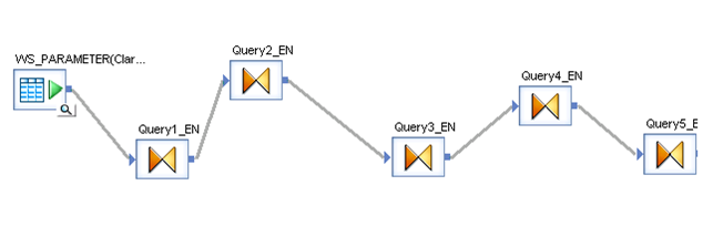
Step 11:
Query 5_EN contains the final result which be two variables that contains the header of the table plus the Load Date.
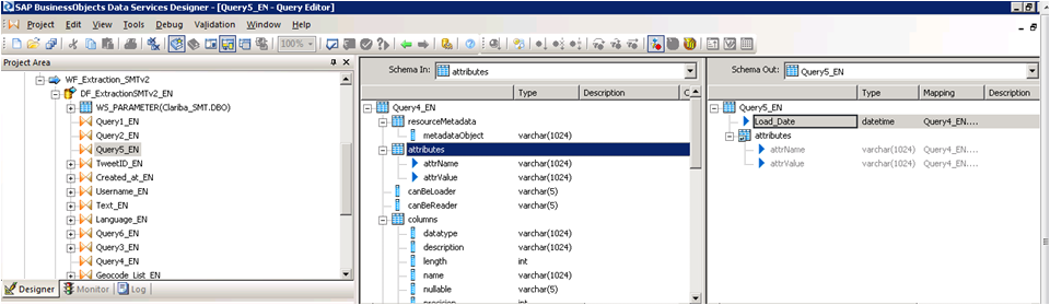
Picture14
Step 12:
The last step depends on the implementation and the business rules. The table returned will have this format.
Column1
Value 1
Column 2
Value 2
Column N...
Value N…
Conclusion
This method applies particularly if you are using function call schema and an array as return type for your web service. If your source is another thing different to an application the resolution of the web Service may vary. The method for mapping the final table is up to you and your business needs. A easy solution could be aggregate an ID to each row.
If you want to have more information please read my previous blogs or leave a comment below.
Spicing up your Dashboard with a clickable moving Ticker
Looking forward to add a little more to your visualizations? Spice them up with a clickable moving ticker! For those who are not familiar with Dashboard Design (formerly known as Xcelsius), a moving ticker is a banner which has a similar look to a stock market ticker displaying customized moving labels from right to left. The one described here is also clickable, which means that when you click on any label it can execute many actions such as opening URL’s.

We always try to build dashboards that people really use, and for that we need to find a balance between functionality and design. The design might not seem as important as the functionality, but trust me, in order to get the attention of users you need to build something that really catches their eyes, such as this ticker feature which is easily noticeable to do it´s constant movement.
Step by step process
In order to help you make your Dashboards eye-catching, I am going to show you how to build a clickable ticker to open URL’s with the following steps.
Let’s start by organizing our spreadsheet (find example below – Fig.1) with the following information:
- Labels: Information that will be displayed on the ticker
- URLs: Links that will be opened when clicking on the labels
- Auxiliary info: cells containing Index, destination, status, key, URL to open, which will be explained later on

When your spreadsheet is ready follow these steps:
1) Drag and Drop the ticker object to your canvas.
The ticker object can be found under the category “Selector”.

2) Configure the Ticker object’s properties.
In the General tab, assign the labels you would like to show on the dashboard.
Insertion type: Position
Destination: This cell is key as it will give the position number of the clicked label on the ticker.
e.g: If you click the third label of the ticker this cell will be a “3”, it it will change when you click another label.

3) Drag and Drop a URL object to your Canvas.
The URL object can be found under the category “Web Conectivity”

4) Configure the URL object’s properties and behavior.
URL: In this cell you need to build a “vlookup” formula as it is shown in fig.1.

In the behavior tab under the Trigger Behavior properties you find:
Trigger cell: This is going to be the same as the destination cell of the Ticker (Sheet1!D$4 in this case – Fig 2.).
Check the “When Value Changes” option.
Hide this button by selecting different values for the status and key cells as below:

The outcome and conclusions
After completing these steps you should have built a clickable moving ticker which will spice up your visualization.
This solution will allow you to:
- Open Intranet/Internet URL’s from moving labels.
- Change visibility dynamically for graphs and images from you Dashboard Design visualization.
- Enhance the design and gain visibility of your visualizations
I hope this feature is useful to you and it brings positive feedback from your end users. Please feel free to leave a comment or question below.
Managing ETL dependencies with SAP BusinessObjects Data Services (Part 2)
Are you satisfied with the way you currently manage the dependencies in your ETL? In part 1 of this article, I talked about the features I’m expecting from a dependency management system, and what are the main possibilities offered (directly or indirectly) by SAP Data Services. Now (part 2 of the article), I’m going to propose an architecture (structure and expected behavior) for a dependency management system inside Data Services. The implementation details will come in part 3, while a feedback on how it went “in real life” as well as possible improvements will come in part 4.
The proposed architecture
What I’m going to develop now is the following: an improvement of the “One job with all processes inside” architecture.
The main features of this architecture are:
- Management of multiple dependencies (one flow can depend on multiple processes)
- Graceful re-start is possible. Full ETL restart is also an option.
We should first create two tables, FLOW_DEPENDENCIES and FLOW_STATUS.
- The table FLOW_DEPENDENCIES has two columns FLOW_NAME and PREREQUISITE. It has one line for each prerequisite.
For the example below (logical flow dependencies in a job)...
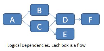
... we would populate the table FLOW_DEPENDENCIES as follows:

Of course you can’t directly implement these logical dependencies in Data Services, so you need to chain them one after the other.

The table is manually updated every time there is a new prerequisite. A flow without prerequisite doesn’t need any row in this table (see flow A for example).
The table FLOW_STATUS keeps track of the different flow statuses (Already run, Success, Failure, Missing Prerequisite) for each execution of the main job. The 3 columns are JOB_KEY (which contains a surrogate key for each new execution of the job), FLOW_NAME and STATUS.
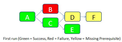
To make things clear, let’s imagine that we run the job for the first time (JOB_KEY = 1).
- Flow A doesn’t have any prerequisite, so it’s allowed to run. It is successful. A row with STATUS = Success is inserted in the FLOW_STATUS table.
- Flow B has a prerequisite according to the table FLOW_DEPENDENCIES (the flow A), so it checks the status of flow A in the same run. It turns out that the flow A was successful, so flow B is allowed to run. Unfortunately, it fails for an unknown reason. A row with STATUS = Failure is inserted in the FLOW_STATUS table.
- Flow C is allowed to run according to the same logic as for flow B. It runs successfully. A row with STATUS = Success is inserted in the FLOW_STATUS table.
- Flow D has two pre-requisites according to the table FLOW_DEPENDENCIES (flows B and C). It checks the status of both. As the flow B failed, the flow D is not allowed to run. A row with STATUS = Missing Prerequisite is inserted in the FLOW_STATUS table.
- Flow E is allowed to run according to the same logic flow B. It runs successfully. A row with STATUS = Success is inserted in the FLOW_STATUS table.
- Flow F has a prerequisite (Flow D). But as the status of flow D is “Missing Prerequisite”, flow F is also not allowed to run. A similar status is inserted in the flow status table.
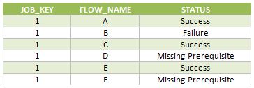
Below are the rows inserted in the FLOW_STATUS table during this job execution.
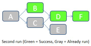
Once the error cause in the flow B has been corrected, we can re-run the job. JOB_KEY will be equal to 2, and we indicate to the job that it should check for statuses of the previous job (in which JOB_KEY = 1).
- The job starts by checking the status of the flow A in the table FLOW_STATUS with JOB_KEY = 1. As the status is equal to Success, the flow A doesn't need to be run in this job. A row with STATUS = “Already run” is inserted in the FLOW_STATUS table.
- Status of flow B with JOB_KEY = 1 is “Failure”. The flow B should accordingly be executed during this job. The job then checks the status of the prerequisite (the flow A) for JOB_KEY = 2. It turns out that the flow A was already run, so flow B is allowed to run. It runs successfully. A row with STATUS = Success is inserted in the FLOW_STATUS table.
- Remaining flows follow a similar logic.
Below are the rows inserted in the FLOW_STATUS table during this job execution.

As you can see, this solution manages the ETL dependencies, keeps trace of the load history, and allows easily a partial re-run of the ETL if a part of it failed. In the next part I’ll give you the details of the Data Services implementation: which scripts/flows/functions/etc. shall we use? How do we make this system easy to implement and maintain? Until then, I’m looking forward to your opinion on this proposed architecture. Does it look good? How would you improve it? Let me know with a comment below.